Welcome to DeepModeling Tutorial!

Hi everyone, here are the tutorials for DeepModeling Projects.

Using DeePMD-Kit

This tutorial tell you how to use DeePMD-kit，for detail information, you can check DeePMD-kit Doc

Introduction

Over the last few decades, molecular dynamics (MD) simulations have attracted much attention due to their wide range of applications in many fields such as condensed matter physics, materials science, polymer chemistry, and molecular biology. They provide researchers access to examine the behavior of atoms or molecules, which is valuable and has the potential to enrich our knowledge, especially when experimentation is difficult, expensive, or even impossible.

It is well recognized that the quality of MD simulations is ultimately limited by the accuracy of the PES and accurately representing the PES is an important challenge in the field of MD simulations. The empirical atomic potential models and the quantum mechanical models have long been two types of models commonly used. The empirical atomic potential models consist of simple low-dimensional terms. They often show excellent computational efficiency, but have limited accuracy. The quantum mechanical models determine the energies and forces on atoms by approximately solving the Schrödinger equation for electronic structure and exhibit higher accuracy. However, quantum mechanical models are computationally demanding, and it is not quite practical for either large-scale or long-time calculations. Overall, a dilemma exists between the choice of an empirical atomic potential model for high efficiency and that of a quantum mechanics model for high accuracy.

Recently, machine-learning (ML) models are emerging as useful tools to address this dilemma. Descriptors and ML algorithms are two main components of the current ML models. The former is used to guarantee the natural symmetries of the system and the latter is used to establish a direct functional relationship between atomic configurations and potential energy by training on reference data generated by quantum mechanics. Once trained, ML models can provide the same accuracy as the quantum mechanical method used to generate the reference data, such as the density functional theory (DFT) accuracy. Meanwhile, the computational cost of DFT scales cubic and that of ML models scale linearly with the size of the system.

So far, different types of ML models have been reported in literatures, such as Behler-Parrinello neural network potentials (BPNNP)[1], Gaussian approximation potentials (GAP)[2], spectral neighbor analysis potentials (SNAP)[3], ANI-1[4], SchNet[5] and Deep Potentials (DP) [6,7,8]. It is worth pointing out that, despite great successes, there are still many challenging issues remaining to be tackled[9]. For example, the neglect of interactions beyond the cut-off radius may lead to systematic prediction errors[10].

This chapter focuses on the DP models. In addition to enabling quantum mechanical accuracy, current DP models also have the following characteristics: (i) ease to preserve the symmetry of the system, especially when there are multiple elemental species; (ii) high computational efficiency, being at least five orders of magnitude faster than DFT; (iii) the model is end-to-end and therefore has little human intervention; (iv) support for MPI and GPU, making it highly efficient on modern heterogeneous high performance supercomputers. Thanks to this, the DP models have been successfully employed in studies of water and water-containing systems[11,12,13,14], metals and alloys[15,16,17,18], phase diagrams[19,20,21], high-entropy ceramics[22,23], chemical reaction[24,25,26], solid-state electrolytes[27], ionic liquids[28], etc. We refer to Ref.[29] for a recent review of DP for materials systems.

Installation

There are various easy methods to install DeePMD-kit. Choose one that you prefer. If you want to build by yourself, jump to the next two sections.

After your easy installation, DeePMD-kit (dp) and LAMMPS (lmp) will be available to execute. You can try dp -h and lmp -h to see the help. mpirun is also available considering you may want to train models or run LAMMPS in parallel.

Install off-line packages
Install with conda
Install with docker

Install off-line packages

Both CPU and GPU version offline packages are available in the Releases page.

Some packages are splited into two files due to size limit of GitHub. One may merge them into one after downloading:

cat deepmd-kit-2.0.0-cuda11.3_gpu-Linux-x86_64.sh.0 deepmd-kit-2.0.0-cuda11.3_gpu-Linux-x86_64.sh.1 > deepmd-kit-2.0.0-cuda11.3_gpu-Linux-x86_64.sh

Install with conda

DeePMD-kit is avaiable with conda. Install Anaconda or Miniconda first.

One may create an environment that contains the CPU version of DeePMD-kit and LAMMPS:

conda create -n deepmd deepmd-kit=*=*cpu libdeepmd=*=*cpu lammps-dp -c https://conda.deepmodeling.org

Or one may want to create a GPU environment containing CUDA Toolkit:

conda create -n deepmd deepmd-kit=*=*gpu libdeepmd=*=*gpu lammps-dp cudatoolkit=11.3 horovod -c https://conda.deepmodeling.org

One could change the CUDA Toolkit version from 10.1 or 11.3.

One may speficy the DeePMD-kit version such as 2.0.0 using

conda create -n deepmd deepmd-kit=2.0.0=*cpu libdeepmd=2.0.0=*cpu lammps-dp=2.0.0 horovod -c https://conda.deepmodeling.org

One may enable the environment using

conda activate deepmd

Install with docker

A docker for installing the DeePMD-kit is available here.

To pull the CPU version:

docker pull ghcr.io/deepmodeling/deepmd-kit:2.0.0_cpu

To pull the GPU version:

docker pull ghcr.io/deepmodeling/deepmd-kit:2.0.0_cuda10.1_gpu

To pull the ROCm version:

docker pull deepmodeling/dpmdkit-rocm:dp2.0.3-rocm4.5.2-tf2.6-lmp29Sep2021

IF you want to Install the DeePMD-kit from source code, please click here.

Theory

Before introducing the DP method, we define the coordinate matrix $\boldsymbol{\mathcal{R}} \in \mathbb{R}^{N \times 3}$ of a system containing $N$ atoms,

$\mathcal{R}=\left\{\boldsymbol{r}_{1}^{T}, \cdots, \boldsymbol{r}_{i}^{T}, \cdots, \boldsymbol{r}_{N}^{T}\right\}^{T}, \boldsymbol{r}_{i}=\left(x_{i}, y_{i}, z_{i}\right),(1)$

$\boldsymbol{r}_{i}$ contains 3 Cartesian coordinates of atom $i$ and $\boldsymbol{\mathcal{R}}$ can be transformed into local environment matrices $\left\{\boldsymbol{\mathcal{R}}^{i}\right\}_{i=1}^{N}$ ,

$\boldsymbol{\mathcal{R}}^{i}=\left\{\boldsymbol{r}_{1 i}^{T}, \cdots, \boldsymbol{r}_{j i}^{T}, \cdots, \boldsymbol{r}_{N_{i}, i}^{T}\right\}^{T}, \boldsymbol{r}_{j i}=\left(x_{j i}, y_{j i}, z_{j i}\right),(2)$

where $j$ and $N_{i}$ are indexes of neighbors of atom $i$ within the cut-off radius $r_{c}$ , and $\boldsymbol{r}_{j i} \equiv \boldsymbol{r}_{j}-\boldsymbol{r}_{i}$ is defined as the relative coordinate.

In the DP method, the total energy $E$ of a system is constructed as a sum of atomic energies.

$E=\sum_{i} E_{i},(3)$

with $E_{i}$ being the local atomic energy of the atom $i$ . $E_{i}$ depends on the local environment of the atom $i$ :

$E=\sum_{i} E_{i}=\sum_{i} E\left(\mathcal{R}^{i}\right),(4)$

The mapping of $\boldsymbol{\mathcal{R}}^{i}$ to $E_{i}$ is constructed in two steps. As seen in figure, $\boldsymbol{\mathcal{R}}^{i}$ is first mapped to a feature matrix, also called the descriptor, $\boldsymbol{\mathcal{D}}^{i}$ to preserve the translational, rotational, and permutational symmetries of the system. $\boldsymbol{\mathcal{R}}^{i} \in \mathbb{R}^{N_{i} \times 3}$ is first transformed into generalized coordinate $\tilde{\boldsymbol{\mathcal{R}}}^{i} \in \mathbb{R}^{N_{i} \times 4}$ .

$\left\{x_{j i}, y_{j i}, z_{j i}\right\} \mapsto\left\{s\left(r_{j i}\right), \hat{x}_{j i}, \hat{y}_{j i}, \hat{z}_{j i}\right\},(5)$

where $\hat{x}_{j i}=\frac{s\left(r_{j i}\right) x_{j i}}{r_{j i}}$ , $\hat{y}_{j i}=\frac{s\left(r_{j i}\right) y_{j i}}{r_{j i}}$ , and $\hat{z}_{j i}=\frac{s\left(r_{j i}\right) z_{j i}}{r_{j i}}$ . $s\left(r_{j i}\right)$ is a weighting function to reduce the weight of particles that are more distant from the atom $i$ , defined as:

$s\left(r_{j i}\right)= \begin{cases}\frac{1}{r_{j i}}, & r_{j i}<r_{c s} \\ \frac{1}{r_{j i}} \{ {(\frac{r_{j i} - r_{c s}}{ r_c - r_{c s}})}^3 (-6 {(\frac{r_{j i} - r_{c s}}{ r_c - r_{c s}})}^2 +15 \frac{r_{j i} - r_{c s}}{ r_c - r_{c s}} -10) +1 \}, & r_{c s}<r_{j i}<r_{c} \\ 0, & r_{j i}>r_{c}\end{cases},(6)$

here $r_{j i}$ is the Euclidean distance between atoms $i$ and $j$ , and $r_{cs}$ is the smooth cutoff parameter. By introducing $s\left(r_{j i}\right)$ the components in $\tilde{\boldsymbol{\mathcal{R}}}^{i}$ smoothly go to zero from $r_{cs}$ to $r_{c}$ . Then $s\left(r_{j i}\right)$ , i.e. the first column of $\tilde{\boldsymbol{\mathcal{R}}}^{i}$ , is mapped to a embedding matrix $\mathcal{G}^{i 2} \in \mathbb{R}^{N_{i} \times M_{1}}$ , through an embedding neural network. By taking the first $M_{2}(<M_{1})$ columns of $\boldsymbol{\mathcal{G}}^{i 2} \in \mathbb{R}^{N_{i} \times M_{2}}$ , we obtain another embedding matrix $\mathcal{G}^{i 2} \in \mathbb{R}^{N_{i} \times M_{2}}$ . Finally, we define the feature matrix $\mathcal{G}^{i 2} \in \mathbb{R}^{M_{1} \times M_{2}}$ of atom $i$ :

$\mathcal{D}^{i}=\left(\mathcal{G}^{i 1}\right)^{T} \tilde{\mathcal{R}}^{i}\left(\tilde{\mathcal{R}}^{i}\right)^{T} \mathcal{G}^{i 2},(7)$

In feature_matrix, translational and rotational symmetries are preserved by the matrix product of $\tilde{\mathcal{R}}^{i}\left(\tilde{\mathcal{R}}^{i}\right)^{T}$ , and permutational symmetry is preserved by the matrix product of $\left(\mathcal{G}^{i}\right)^{T} \tilde{\mathcal{R}}^{i}$ . Next, each $\boldsymbol{\mathcal{D}}^{i}$ is mapped to a local atomic energy $E_{i}$ through a fitting network.

Both the embedding network $\mathcal{N}^e$ and fitting network $\mathcal{N}^f$ are feed-forward neural networks containing several hidden layers. The mapping from input data $d_{l}^{\mathrm{in}}$ of the previous layer to output data $d_{k}^{\mathrm{out}}$ of the next layeris composed of a linear and a non-linear transformation.

$d_{k}^{o u t}=\varphi\left(\sum_{k l} w_{k l} d_{l}^{i n}+ b_{k}\right),(8)$

In Eq.(8), ${w}_{k l}$ is the connecting weight, ${b}_{k}$ the bias weight, and $\varphi$ is a non-linear activation function. It needs to be noted that only linear transformations are applied at the output nodes. The parameters contained in the embedding and fitting networks are obtained by minimizing the loss function $L$ :

$L\left(p_{\epsilon}, p_{f}, p_{\xi}\right)=\frac{p_{\epsilon}}{N} \Delta \epsilon^{2}+\frac{p_{f}}{3 N} \sum_{i}\left|\Delta \boldsymbol{F}_{i}\right|^{2}+\frac{p_{\xi}}{9N}\|\Delta \xi\|^{2},(9)$

where $\Delta \epsilon$ , $\Delta \boldsymbol{F}_{i}$ , and $\Delta \xi$ denote root mean square error (RMSE) in energy, force, and virial, respectively. During the training process, the prefactors $p_{\epsilon}$ , $p_{f}$ , and $p_{\xi}$ are determined by

$p(t)=p^{\operatorname{limit}}\left[1-\frac{r_{l}(t)}{r_{l}^{0}}\right]+p^{\operatorname{start}}\left[\frac{r_{l}(t)}{r_{l}^{0}}\right],(10)$

where $r_{l}(t)$ and $r_{l}^{0}$ are the learning rate at training step $t$ and training step 0. $r_{l}(t)$ is defined as

$r_{l}(t)=r_{l}^{0} \times d_{r}^{t / d_{s}},(11)$

where $d_{r}$ and $d_{s}$ are the decay rate and decay steps, respectively. The decay rate $d_{r}$ is required to be less than 1. The reader is referred to the original papers of DeepPot-SE (DP) method for details.

How to Setup a DeePMD-kit Training within 5 Minutes

DeePMD-kit is a software to implement Deep Potential. There is a lot of information on the Internet, but there are not so many tutorials for the new hand, and the official guide is too long. Today, I’ll take you 5 minutes to get started with DeePMD-kit.

Let’s take a look at the training process of DeePMD-kit:

Prepare data –> Training –> Freeze/Compress the model

What? Only three steps? Yes, it’s that simple.

Preparing data is converting the computational results of DFT to data that can be recognized by the DeePMD-kit.
Training is train a Deep Potential model using the DeePMD-kit with data prepared in the previous step.
Finally, what we need to do is to freeze/compress the restart file in the training process into a model. I believe you can’t wait to get started. Let’s go!

Tutorial Data

First, let’s download and decompress the tutorial data:

    $ wget https://dp-public.oss-cn-beijing.aliyuncs.com/community/DeePMD-kit-FastLearn.tar
    $ tar xvf DeePMD-kit-FastLearn.tar

Then we can go to the Tutorial data and have a look:

    $ cd DeePMD-kit-FastLearn
    $ ls
    00.data 01.train data

Three directories are set for different purpose:

00.data: contains an example of VASP result OUTCAR
01.train: contains an example of DeePMD-kit configuration input.json
data: contains an example of DeePMD-kit training/validation data

Preparing Data

Now Let’s go into 00.data directory:

    $ cd 00.data
    $ ls
    OUTCAR

This file OUTCAR is the computational result of the VASP. We need convert it into DeePMD-kit format. The data format of the DeePMD-kit is introduced in the official document but seems complex. Don’t worry, I’d like to introduce a data processing tool: dpdata! You can use only one line Python scripts to process data. So easy!

   import dpdata
   dpdata.LabeledSystem('OUTCAR').to('deepmd/npy', 'data', set_size=200)

In this example, we converted the computational results of the VASP in the OUTCAR to the data format of the DeePMD-kit and saved in to a directory named data, where npy is the compressed format of the numpy, which is required by the DeePMD-kit training.

Suppose you have an “OUTCAR” for molecular dynamics, which contains 1000 frames.set_size=200 means these 1000 points will be divided into 5 subsets, which is named as data/set.000~data/set.004, respectively. The size of each set is 200. In these 5 sets, data/set.000~data/set.003 will be considered as the training set by the DeePMD-kit, and data/set.004 will be considered as the test set. The last set will be considered as the test set by the DeePMD-kit by default. If there is only one set, the set will be both the training set and the test set. (Of course, such test set is meaningless.)

“OUTCAR” we provided only contains 1 frame, so in “data” directory(in the same directory with “OUTCAR”) there is only 1 set: data/set.000. Some procudure needs to be done if you want to use these data. Detailed method using dpdata can be found in next chapter.

Now we just skip these details and use the data we prepared for you. The data is in the root directory of our Tutorial data.

    $ cd ..
    $ ls
    00.data 01.train data

Training

It’s required to prepare an input script to start the DeePMD-kit training. Are you still out of the fear of being dominated by INCAR script? Don’t worry, it’s much easier to configure the DeePMD-kit than configuring the VASP.We have prepared input.json for you, you can find it in “01.train” directory:

   $ cd 01.train
   $ ls
   input.json

The strength of the DeePMD-kit is that the same training parameters are suitable for different systems, so we only need to slightly modify input.json to start training. Here is the first parameter to modify:

   "type_map":     ["O", "H"],

In the DeePMD-kit data, each atom type is numbered as an integer starting from 0. The parameter gives an element name to each atom in the numbering system. Here, we can copy from the content of data/type_map.raw. For example,

   "type_map":    ["A", "B","C"],

Next, we are going to modify the neighbour searching parameter:

   "sel":       [46, 92],

Each number in this list gives the maximum number of atoms of each type among neighbor atoms of an atom. For example, 46 means there are at most 46 O (type 0) neighbours. Here, our elements were modified to A, B, and C, so this parameters is also required to modify. What to do if you don’t know the maximum number of neighbors? You can be roughly estimate one by the density of the system, or try a number blindly. If it is not big enough, the DeePMD-kit will shoot WARNINGS. Below we changed it to

   "sel":       [64, 64, 64]

In addtion, we need to modify "systems" in "training_data"

   "training_data":{
          "systems":     ["../data/data_0/", "../data/data_1/", "../data/data_2/"],

and "validation_data"

   "validation_data":{
          "systems":     ["../data/data_3"],

Here I’d like to introduce the definition of the data system. The DeePMD-kit considers that data with corresponding element types and atomic numbers form a system. If data cannot be put into a system, multiple systems is required to be set as a list here:

   "systems": ["system1", "system2"]

Finnally, we are likely to modify another parameter:

   "numb_steps":   1000,

numb_steps is the numebr of training step using the SGD method of deep learning.(It is only an example, you should set a larger number in practice)

Now we have succesfully set a input file! To start training, we execuate

   dp train input.json

and wait for results. During the training process, we can see lcurve.out to observe the error reduction.Among them, Column 4 and 5 are the test and training errors of energy (normalized by the number of atoms), and Column 6 and 7 are the test and training errors of the force.

Freeze/Compress the Model

After training, we can use the following script to freeze the model:

   dp freeze -o graph.pb

The default filename of the output model is graph.pb. And we can use the following script to compress the model:

   dp compress -i graph.pb -o graph-compress.pb

As so, we have got a good or bad DP model. As for the reliability of this model and how to use it, I will give you a detailed tutorial in the next post.

Handson-Tutorial(v2.0.3)

This tutorial will introduce you to the basic usage of the DeePMD-kit, taking a gas phase methane molecule as an example. Typically the DeePMD-kit workflow contains three parts:

Data preparation
Training/Freezing/Compressing/Testing
Molecular dynamics

The DP model is generated using the DeePMD-kit package (v2.0.3). The training data is converted into the format of DeePMD-kit using a tool named dpdata (v0.2.5). It needs to be noted that dpdata only works with Python 3.5 and later versions. The MD simulations are carried out using LAMMPS (29 Sep 2021) integrated with DeePMD-kit. Details of dpdata and DeePMD-kit installation and execution of can be found in the DeepModeling official GitHub site. OVITO is used for the visualization of the MD trajectory.

The files needed for this tutorial are available.

    $ wget https://dp-public.oss-cn-beijing.aliyuncs.com/community/CH4.tar
    $ tar xvf CH4.tar

The folder structure of this tutorial is like this:

$ cd CH4
$ ls
00.data 01.train 02.lmp

There are 3 folders here:

The folder 00.data contains the data
The folder 01.train contains an example input script to train a model with DeePMD-kit
The folder 02.lmp contains LAMMPS example script for molecular dynamics simulation

Data preparation

The training data of the DeePMD-kit contains the atom type, the simulation box, the atom coordinate, the atom force, the system energy, and the virial. A snapshot of a molecular system that has this information is called a frame. A system of data includes many frames that share the same number of atoms and atom types. For example, a molecular dynamics trajectory can be converted into a system of data, with each time step corresponding to a frame in the system.

The DeePMD-kit adopts a compressed data format. All training data should first be converted into this format and can then be used by DeePMD-kit. The data format is explained in detail in the DeePMD-kit manual that can be found in the DeePMD-kit official Github site .

We provide a convenient tool named dpdata for converting the data produced by VASP, Gaussian, Quantum-Espresso, ABACUS, and LAMMPS into the compressed format of DeePMD-kit.

As an example, go to the data folder:

$ cd 00.data
$ ls 
OUTCAR

The OUTCAR was produced by an ab-initio molecular dynamics (AIMD) simulation of a gas phase methane molecule using VASP. Now start an interactive python environment, for example

$ python

then execute the following commands:

import dpdata 
import numpy as np
data = dpdata.LabeledSystem('OUTCAR', fmt = 'vasp/outcar') 
print('# the data contains %d frames' % len(data))

On the screen, you can see that the OUTCAR file contains 200 frames of data. We randomly pick 40 frames as validation data and the rest as training data.

index_validation = np.random.choice(200,size=40,replace=False)     # random choose 40 index for validation_data
index_training = list(set(range(200))-set(index_validation))       # other indexes are training_data
data_training = data.sub_system(index_training)
data_validation = data.sub_system(index_validation)
data_training.to_deepmd_npy('training_data')               # all training data put into directory:"training_data" 
data_validation.to_deepmd_npy('validation_data')           # all validation data put into directory:"validation_data"
print('# the training data contains %d frames' % len(data_training)) 
print('# the validation data contains %d frames' % len(data_validation)) 

The commands import a system of data from the OUTCAR (with format vasp/outcar ), and then dump it into the compressed format (numpy compressed arrays). The data in DeePMD-kit format is stored in the folder 00.data. Lets have a look:

    $ ls 
    OUTCAR training_data validation_data

The directories “training_data” and “validation_data” have similar structure, so we just explain “training_data”:

$ ls training_data
set.000 type.raw type_map.raw

set.000: is a directory, contains data in compressed format (numpy compressed arrays).
type.raw: is a file, contains types of atoms(Represented in integer)
type_map.raw: is a file, contains type name of atoms.

Lets have a look at type.raw:

    $ cat training_data/type.raw 
    0 0 0 0 1

This tells us there are 5 atoms in this example, 4 atoms represented by type “0”, and 1 atom represented by type “1”. Sometimes one needs to map the integer types to atom name. The mapping can be given by the file type_map.raw

$ cat training_data/type_map.raw 
H C

This tells us the type “0” is named by “H”, and the type “1” is named by “C”.

More detailed doc about Data conversion can be found here

Training

Prepare input script

Once the data preparation is done, we can go on with training. Now go to the training directory

$ cd ../01.train
$ ls 
input.json

where input.json gives you an example training script. The options are explained in detail in the DeePMD-kit manual, so they are not comprehensively explained.

In the model section, the parameters of embedding and fitting networks are specified.

"model":{
    "type_map":    ["H", "C"],                           # the name of each type of atom
    "descriptor":{
        "type":            "se_e2_a",                    # full relative coordinates are used
        "rcut":            6.00,                         # cut-off radius
        "rcut_smth":       0.50,                         # where the smoothing starts
        "sel":             [4, 1],                       # the maximum number of type i atoms in the cut-off radius
        "neuron":          [10, 20, 40],                 # size of the embedding neural network
        "resnet_dt":       false,
        "axis_neuron":     4,                            # the size of the submatrix of G (embedding matrix)
        "seed":            1,
        "_comment":        "that's all"
    },
    "fitting_net":{
        "neuron":          [100, 100, 100],              # size of the fitting neural network
        "resnet_dt":       true,
        "seed":            1,
        "_comment":        "that's all"
    },
    "_comment":    "that's all"'
},

The se\_e2\_a descriptor is used to train the DP model. The item neurons set the size of the embedding and fitting network to [10, 20, 40] and [100, 100, 100], respectively. The components in $\tilde{\mathcal{R}}^{i}$ to smoothly go to zero from 0.5 to 6 Å.

The following are the parameters that specify the learning rate and loss function.

    "learning_rate" :{
        "type":                "exp",
        "decay_steps":         5000,
        "start_lr":            0.001,    
        "stop_lr":             3.51e-8,
        "_comment":            "that's all"
    },
    "loss" :{
        "type":                "ener",
        "start_pref_e":        0.02,
        "limit_pref_e":        1,
        "start_pref_f":        1000,
        "limit_pref_f":        1,
        "start_pref_v":        0,
        "limit_pref_v":        0,
        "_comment":            "that's all"
},

In the loss function, pref\_e increases from 0.02 to 1 $\mathrm{eV}^{-2}$ , and pref\_f decreases from 1000 to 1 $\AA^{2} \mathrm{eV}^{-2}$ progressively, which means that the force term dominates at the beginning, while energy and virial terms become important at the end. This strategy is very effective and reduces the total training time. pref_v is set to 0 $\mathrm{eV}^{-2}$ , indicating that no virial data are included in the training process. The starting learning rate, stop learning rate, and decay steps are set to 0.001, 3.51e-8, and 5000, respectively. The model is trained for $10^6$ steps.

The training parameters are given in the following

    "training" : {
        "training_data": {
            "systems":            ["../00.data/training_data"],     
            "batch_size":         "auto",                       
            "_comment":           "that's all"
        },
        "validation_data":{
            "systems":            ["../00.data/validation_data/"],
            "batch_size":         "auto",               
            "numb_btch":          1,
            "_comment":           "that's all"
        },
        "numb_steps":             100000,                           
        "seed":                   10,
        "disp_file":              "lcurve.out",
        "disp_freq":              1000,
        "save_freq":              10000,
    },

Train a model

After the training script is prepared, we can start the training with DeePMD-kit by simply running

$ dp train input.json

On the screen, you see the information of the data system(s)

DEEPMD INFO      ----------------------------------------------------------------------------------------------------
DEEPMD INFO      ---Summary of DataSystem: training     -------------------------------------------------------------
DEEPMD INFO      found 1 system(s):
DEEPMD INFO                              system        natoms        bch_sz        n_bch          prob        pbc
DEEPMD INFO           ../00.data/training_data/             5             7           22         1.000          T
DEEPMD INFO      -----------------------------------------------------------------------------------------------------
DEEPMD INFO      ---Summary of DataSystem: validation   --------------------------------------------------------------
DEEPMD INFO      found 1 system(s):
DEEPMD INFO                               system       natoms        bch_sz        n_bch          prob        pbc
DEEPMD INFO          ../00.data/validation_data/            5             7            5         1.000          T

and the starting and final learning rate of this training

DEEPMD INFO      start training at lr 1.00e-03 (== 1.00e-03), decay_step 5000, decay_rate 0.950006, final lr will be 3.51e-08

If everything works fine, you will see, on the screen, information printed every 1000 steps, like

DEEPMD INFO    batch    1000 training time 7.61 s, testing time 0.01 s
DEEPMD INFO    batch    2000 training time 6.46 s, testing time 0.01 s
DEEPMD INFO    batch    3000 training time 6.50 s, testing time 0.01 s
DEEPMD INFO    batch    4000 training time 6.44 s, testing time 0.01 s
DEEPMD INFO    batch    5000 training time 6.49 s, testing time 0.01 s
DEEPMD INFO    batch    6000 training time 6.46 s, testing time 0.01 s
DEEPMD INFO    batch    7000 training time 6.24 s, testing time 0.01 s
DEEPMD INFO    batch    8000 training time 6.39 s, testing time 0.01 s
DEEPMD INFO    batch    9000 training time 6.72 s, testing time 0.01 s
DEEPMD INFO    batch   10000 training time 6.41 s, testing time 0.01 s
DEEPMD INFO    saved checkpoint model.ckpt

They present the training and testing time counts. At the end of the 10000th batch, the model is saved in Tensorflow’s checkpoint file model.ckpt. At the same time, the training and testing errors are presented in file lcurve.out. The file contains 8 columns, form left to right, are the training step, the validation loss, training loss, root mean square (RMS) validation error of energy, RMS training error of energy, RMS validation error of force, RMS training error of force and the learning rate. The RMS error (RMSE) of the energy is normalized by number of atoms in the system.

$ head -n 2 lcurve.out
#step       rmse_val       rmse_trn       rmse_e_val       rmse_e_trn       rmse_f_val       rmse_f_trn           lr
0           1.34e+01       1.47e+01         7.05e-01         7.05e-01         4.22e-01         4.65e-01     1.00e-03

and

$ tail -n 2 lcurve.out
999000      1.24e-01       1.12e-01         5.93e-04         8.15e-04         1.22e-01         1.10e-01      3.7e-08
1000000     1.31e-01       1.04e-01         3.52e-04         7.74e-04         1.29e-01         1.02e-01      3.5e-08

Volumes 4, 5 and 6, 7 present energy and force training and testing errors, respectively. It is demonstrated that after 140,000 steps of training, the energy testing error is less than 1 meV and the force testing error is around 120 meV/Å. It is also observed that the force testing error is systematically (but slightly) larger than the training error, which implies a slight over-fitting to the rather small dataset.

One can visualize this file by a simple Python script:

import numpy as np
import matplotlib.pyplot as plt

data = np.genfromtxt("lcurve.out", names=True)
for name in data.dtype.names[1:-1]:
    plt.plot(data['step'], data[name], label=name)
plt.legend()
plt.xlabel('Step')
plt.ylabel('Loss')
plt.xscale('symlog')
plt.yscale('log')
plt.grid()
plt.show()

When the training process is stopped abnormally, we can restart the training from the provided checkpoint by simply running

$ dp train  --restart model.ckpt  input.json

In the lcurve.out, you can see the training and testing errors, like

538000      3.12e-01       2.16e-01         6.84e-04         7.52e-04         1.38e-01         9.52e-02      4.1e-06
538000      3.12e-01       2.16e-01         6.84e-04         7.52e-04         1.38e-01         9.52e-02      4.1e-06
539000      3.37e-01       2.61e-01         7.08e-04         3.38e-04         1.49e-01         1.15e-01      4.1e-06
 #step      rmse_val       rmse_trn       rmse_e_val       rmse_e_trn       rmse_f_val       rmse_f_trn           lr
530000      2.89e-01       2.15e-01         6.36e-04         5.18e-04         1.25e-01         9.31e-02      4.4e-06
531000      3.46e-01       3.26e-01         4.62e-04         6.73e-04         1.49e-01         1.41e-01      4.4e-06

Note that input.json needs to be consistent with the previous one.

Freeze and Compress a model

At the end of the training, the model parameters saved in TensorFlow’s checkpoint file should be frozen as a model file that is usually ended with extension .pb. Simply execute

$ dp freeze -o graph.pb
DEEPMD INFO    Restoring parameters from ./model.ckpt-1000000
DEEPMD INFO    1264 ops in the final graph

and it will output a model file named graph.pb in the current directory. The compressed DP model typically speed up DP-based calculations by an order of magnitude faster, and consume an order of magnitude less memory. The graph.pb can be compressed in the following way:

$ dp compress -i graph.pb -o graph-compress.pb
DEEPMD INFO    stage 1: compress the model
DEEPMD INFO    built lr
DEEPMD INFO    built network
DEEPMD INFO    built training
DEEPMD INFO    initialize model from scratch
DEEPMD INFO    finished compressing
DEEPMD INFO    
DEEPMD INFO    stage 2: freeze the model
DEEPMD INFO    Restoring parameters from model-compression/model.ckpt
DEEPMD INFO    840 ops in the final graph

and it will output a model file named graph-compress.pb.

Test a model

We can check the quality of the trained model by running

$ dp test -m graph-compress.pb -s ../00.data/validation_data -n 40 -d results

On the screen you see the information of the prediction errors of validation data

    DEEPMD INFO    # number of test data    : 40 
    DEEPMD INFO    Energy RMSE              : 3.168050e-03 eV
    DEEPMD INFO    Energy RMSE/Natoms       : 6.336099e-04 eV
    DEEPMD INFO    Force  RMSE              : 1.267645e-01 eV/A
    DEEPMD INFO    Virial RMSE              : 2.494163e-01 eV
    DEEPMD INFO    Virial RMSE/Natoms       : 4.988326e-02 eV
    DEEPMD INFO    # ----------------------------------------------- 

and it will output files named results.e.out and results.f.out in the current directory.

Run MD with LAMMPS

Now let’s switch to the lammps directory to check the necessary input files for running DeePMD with LAMMPS.

$ cd ../02.lmp

Firstly, we soft-link the output model in the training directory to the current directory

$ ln -s ../01.train/graph-compress.pb

Then we have three files

$ ls
conf.lmp  graph-compress.pb  in.lammps

where conf.lmp gives the initial configuration of a gas phase methane MD simulation, and the file in.lammps is the lammps input script. One may check in.lammps and finds that it is a rather standard LAMMPS input file for a MD simulation, with only two exception lines:

pair_style  graph-compress.pb
pair_coeff  * *

where the pair style deepmd is invoked and the model file graph-compress.pb is provided, which means the atomic interaction will be computed by the DP model that is stored in the file graph-compress.pb.

One may execute lammps in the standard way

$ lmp  -i  in.lammps

After waiting for a while, the MD simulation finishes, and the log.lammps and ch4.dump files are generated. They store thermodynamic information and the trajectory of the molecule, respectively. One may want to visualize the trajectory by, e.g. OVITO

$ ovito ch4.dump

to check the evolution of the molecular configuration.

Using DP-GEN

This tutorial tell you how to use DP-GEN，for detail information, you can check DP-GEN Doc

Hands-on tutorial for DP-GEN (v0.10.3)

Writer: Wenshuo Liang

Verifier: Yibo Wang

General Introduction

Deep Potential GENerator (DP-GEN) is a package that implements a concurrent learning scheme to generate reliable DP models. Typically, the DP-GEN workflow contains three processes: init, run, and autotest.

init: generate the initial training dataset by first-principle calculations.
run: the main process of DP-GEN, in which the training dataset is enriched and the quality of the DP models is improved automatically.
autotest: calculate a simple set of properties and/or perform tests for comparison with DFT and/or empirical interatomic potentials.

This is a practical tutorial that aims to help you quickly get command of dpgen run interface.

Input files

In this tutorial, we take a gas-phase methane molecule as an example. We have prepared input files in dpgen_example/run

Now download the dpgen_example and uncompress it:

wget https://dp-public.oss-cn-beijing.aliyuncs.com/community/dpgen_example.tar.xz
tar xvf dpgen_example.tar.xz

Now go into the dpgen_example/run.

$ cd dpgen_example/run
$ ls
INCAR_methane  machine.json  param.json  POTCAR_C  POTCAR_H

param.json is the settings for DP-GEN for the current task. It will expalin later.
machine.json is a task dispatcher where the machine environment and resource requirements are set.We have expalined here
INCAR* and POTCAR* are the input file for the VASP package. All first-principle calculations share the same parameters as the one you set in param.json.

Run process

We can run DP-GEN easily by:

$ dpgen run param.json machine.json

The run process contains a series of successive iterations. Each iteration is composed of three steps:

exploration
labeling
training

Accordingly, there are three sub-folders in each iteration:

00.train
01.model_devi
02.fp

param.json

We provide an example of param.json.

{
     "type_map": ["H","C"],
     "mass_map": [1,12],
     "init_data_prefix": "../",
     "init_data_sys": ["init/CH4.POSCAR.01x01x01/02.md/sys-0004-0001/deepmd"],
     "sys_configs_prefix": "../",
     "sys_configs": [
         ["init/CH4.POSCAR.01x01x01/01.scale_pert/sys-0004-0001/scale/00000/POSCAR"],
         ["init/CH4.POSCAR.01x01x01/01.scale_pert/sys-0004-0001/scale/00001/POSCAR"]
     ],
     "_comment": " that's all ",
     "numb_models": 4,
     "default_training_param": {
         "model": {
             "type_map": ["H","C"],
             "descriptor": {
                 "type": "se_a",
                 "sel": [16,4],
                 "rcut_smth": 0.5,
                 "rcut": 5.0,
                 "neuron": [120,120,120],
                 "resnet_dt": true,
                 "axis_neuron": 12,
                 "seed": 1
             },
             "fitting_net": {
                 "neuron": [25,50,100],
                 "resnet_dt": false,
                 "seed": 1
             }
         },
         "learning_rate": {
             "type": "exp",
             "start_lr": 0.001,
             "decay_steps": 5000
         },
         "loss": {
             "start_pref_e": 0.02,
             "limit_pref_e": 2,
             "start_pref_f": 1000,
             "limit_pref_f": 1,
             "start_pref_v": 0.0,
             "limit_pref_v": 0.0
         },
         "training": {
             "stop_batch": 400000,
             "disp_file": "lcurve.out",
             "disp_freq": 1000,
             "numb_test": 4,
             "save_freq": 1000,
             "save_ckpt": "model.ckpt",
             "disp_training": true,
             "time_training": true,
             "profiling": false,
             "profiling_file": "timeline.json",
             "_comment": "that's all"
         }
     },
     "model_devi_dt": 0.002,
     "model_devi_skip": 0,
     "model_devi_f_trust_lo": 0.05,
     "model_devi_f_trust_hi": 0.15,
     "model_devi_e_trust_lo": 10000000000.0,
     "model_devi_e_trust_hi": 10000000000.0,
     "model_devi_clean_traj": true,
     "model_devi_jobs": [
         {"sys_idx": [0],"temps": [100],"press": [1.0],"trj_freq": 10,"nsteps": 300,"ensemble": "nvt","_idx": "00"},
         {"sys_idx": [1],"temps": [100],"press": [1.0],"trj_freq": 10,"nsteps": 3000,"ensemble": "nvt","_idx": "01"}
     ],
     "fp_style": "vasp",
     "shuffle_poscar": false,
     "fp_task_max": 20,
     "fp_task_min": 5,
     "fp_pp_path": "./",
     "fp_pp_files": ["POTCAR_H","POTCAR_C"],
     "fp_incar": "./INCAR_methane"
}

The following is a detailed description of the keywords.

Basics keywords (Line 2-3):

Key	Type	Description
“type_map”	List of string	Atom types
“mass_map”	List of float	Standard atom weights.

Data-related keywords (Line 4-10):

Key	Type	Description
“init_data_prefix”	String	Prefix of initial data directories
“init_data_sys”	List of string	Directories of initial data. You may use either absolute or relative path here.
“sys_configs_prefix”	String	Prefix of sys_configs
“sys_configs”	List of string	Containing directories of structures to be explored in iterations. Wildcard characters are supported here.

Training-related keywords (Line 12-58):

Key	Type	Description
“numb_models”	Integer	Number of models to be trained in 00.train.
“default_training_param”	Dict	Training parameters for deepmd-kit.

Exploration-related keywords (Line 59-69):

Key	Type	Description
“model_devi_dt”	Float	Timestep for MD
“model_devi_skip”	Integer	Number of structures skipped for fp in each MD
“model_devi_f_trust_lo”	Float	Lower bound of forces for the selection. If List, should be set for each index in sys_configs, respectively.
“model_devi_f_trust_hi”	Integer	Upper bound of forces for the selection. If List, should be set for each index in sys_configs, respectively.
“model_devi_f_trust_hi”	Float or List of float	Lower bound of virial for the selection. If List, should be set for each index in sys_configs, respectively. Should be used with DeePMD-kit v2.x.
“model_devi_f_trust_hi”	Float or List of float	Upper bound of virial for the selection. If List, should be set for each index in sys_configs, respectively. Should be used with DeePMD-kit v2.x.
“model_devi_clean_traj”	Boolean or Int	If type of model_devi_clean_traj is boolean type then it denote whether to clean traj folders in MD since they are too large. If it is Int type, then the most recent n iterations of traj folders will be retained, others will be removed.
“model_devi_jobs”	List of Dict	Settings for exploration in 01.model_devi. Each dict in the list corresponds to one iteration. The index of model_devi_jobs exactly accord with index of iterations

Labeling-related parameters (Line 70-76):

Key	Type	Description
“fp_style”	String	Software for First Principles. Options include “vasp”, “pwscf”, “siesta” and “gaussian” up to now.
“shuffle_poscar”	Boolean
“fp_task_max”	Integer	Maximum of structures to be calculated in 02.fp of each iteration.
“fp_task_min”	Integer	Minimum of structures to calculate in 02.fp of each iteration.
“fp_pp_path”	String	Directory of psuedo-potential file to be used for 02.fp exists.
“fp_pp_files”	List of string	Psuedo-potential file to be used for 02.fp. Note that the order of elements should correspond to the order in type_map.
“fp_incar”	String	Input file for VASP. INCAR must specify KSPACING and KGAMMA.

Output files

In dpgen_example/run, we can find that a folder and two files are generated automatically.

$ ls 
dpgen.log  INCAR_methane  iter.000000  machine.json  param.json  record.dpgen 

iter.000000 contains the main results that DP-GEN generates in the first iteration.
record.dpgen records the current stage of the run process.
dpgen.log includes time and iteration information. When the first iteration is completed, the folder structure of iter.000000 is like this:

$ tree iter.000000/ -L 1
./iter.000000/
├── 00.train
├── 01.model_devi
└── 02.fp

00.train

First, we check the folder iter.000000/ 00.train.

$ tree iter.000000/00.train -L 1
./iter.000000/00.train/
├── 000
├── 001
├── 002
├── 003
├── data.init -> /root/dpgen_example
├── data.iters
├── graph.000.pb -> 000/frozen_model.pb
├── graph.001.pb -> 001/frozen_model.pb
├── graph.002.pb -> 002/frozen_model.pb
└── graph.003.pb -> 003/frozen_model.pb

Folder 00x contains the input and output files of the DeePMD-kit, in which a model is trained.
graph.00x.pb , linked to 00x/frozen.pb, is the model DeePMD-kit generates. The only difference between these models is the random seed for neural network initialization. We may randomly select one of them, like 000.

$ tree iter.000000/00.train/000 -L 1
./iter.000000/00.train/000
├── checkpoint
├── frozen_model.pb
├── input.json
├── lcurve.out
├── model.ckpt-400000.data-00000-of-00001
├── model.ckpt-400000.index
├── model.ckpt-400000.meta
├── model.ckpt.data-00000-of-00001
├── model.ckpt.index
├── model.ckpt.meta
└── train.log

input.json is the settings for deepmd-kit for current task.
checkpoint is used for restart traning.
model.ckpt* are model related files.
frozen_model.pb is the frozen model.
lcurve.out records the training accuracy of energies and forces.
train.log includes version, data, hardware information, time, etc.

01.model_devi

Then, we check the folder iter.000000/ 01.model_devi.

$ tree iter.000000/01.model_devi -L 1
./iter.000000/01.model_devi/
├── confs
├── graph.000.pb -> /root/dpgen_example/run/iter.000000/00.train/graph.000.pb
├── graph.001.pb -> /root/dpgen_example/run/iter.000000/00.train/graph.001.pb
├── graph.002.pb -> /root/dpgen_example/run/iter.000000/00.train/graph.002.pb
├── graph.003.pb -> /root/dpgen_example/run/iter.000000/00.train/graph.003.pb
├── task.000.000000
├── task.000.000001
├── task.000.000002
├── task.000.000003
├── task.000.000004
├── task.000.000005
├── task.000.000006
├── task.000.000007
├── task.000.000008
└── task.000.000009

Folder confs contains the initial configurations for LAMMPS MD converted from POSCAR you set in “sys_configs” of param.json.
Folder task.000.00000x contains the input and output files of the LAMMPS. We may randomly select one of them, like task.000.000001.

$ tree iter.000000/01.model_devi/task.000.000001
./iter.000000/01.model_devi/task.000.000001
├── conf.lmp -> ../confs/000.0001.lmp
├── input.lammps
├── log.lammps
├── model_devi.log
└── model_devi.out

conf.lmp, linked to 000.0001.lmp in folder confs, serves as the initial configuration of MD.
input.lammps is the input file for LAMMPS.
model_devi.out records the model deviation of concerned labels, energy and force, in MD. It serves as the criterion for selecting which structures and doing first-principle calculations.

By head model_devi.out, you will see:

$ head -n 5 ./iter.000000/01.model_devi/task.000.000001/model_devi.out
 #  step max_devi_v     min_devi_v     avg_devi_v     max_devi_f     min_devi_f     avg_devi_f 
 0     1.438427e-04   5.689551e-05   1.083383e-04   8.835352e-04   5.806717e-04   7.098761e-04
10     3.887636e-03   9.377374e-04   2.577191e-03   2.880724e-02   1.329747e-02   1.895448e-02
20     7.723417e-04   2.276932e-04   4.340100e-04   3.151907e-03   2.430687e-03   2.727186e-03
30     4.962806e-03   4.943687e-04   2.925484e-03   5.866077e-02   1.719157e-02   3.011857e-02

Now we’ll concentrate on max_devi_f. Recall that we’ve set "trj_freq" as 10, so every 10 steps the structures are saved. Whether to select the structure depends on its "max_devi_f". If it falls between "model_devi_f_trust_lo" (0.05) and "model_devi_f_trust_hi" (0.15), DP-GEN will treat the structure as a candidate. Here, only the 30th structure will be selected, whose "max_devi_f" is 5.866077e e-02.

02.fp

Finally, we check the folder iter.000000/ 02.fp.

$ tree iter.000000/02.fp -L 1
./iter.000000/02.fp
├── data.000
├── task.000.000000
├── task.000.000001
├── task.000.000002
├── task.000.000003
├── task.000.000004
├── task.000.000005
├── task.000.000006
├── task.000.000007
├── task.000.000008
├── task.000.000009
├── task.000.000010
├── task.000.000011
├── candidate.shuffled.000.out
├── POTCAR.000
├── rest_accurate.shuffled.000.out
└── rest_failed.shuffled.000.out

POTCAR is the input file for VASP generated according to "fp_pp_files" of param.json.
candidate.shuffle.000.out records which structures will be selected from last step 01.model_devi. There are always far more candidates than the maximum you expect to calculate at one time. In this condition, DP-GEN will randomly choose up to "fp_task_max" structures and form the folder task.*.
rest_accurate.shuffle.000.out records the other structures where our model is accurate (“max_devi_f” is less than "model_devi_f_trust_lo", no need to calculate any more),
rest_failed.shuffled.000.out records the other structures where our model is too inaccurate (lager than "model_devi_f_trust_hi", there may be some error).
data.000: After first-principle calculations, DP-GEN will collect these data and change them into the format DeePMD-kit needs. In the next iteration’s 00.train, these data will be trained together as well as initial data.

By cat candidate.shuffled.000.out | grep task.000.000001, you will see:

$ cat ./iter.000000/02.fp/candidate.shuffled.000.out | grep task.000.000001
iter.000000/01.model_devi/task.000.000001 190
iter.000000/01.model_devi/task.000.000001 130
iter.000000/01.model_devi/task.000.000001 120
iter.000000/01.model_devi/task.000.000001 150
iter.000000/01.model_devi/task.000.000001 280
iter.000000/01.model_devi/task.000.000001 110
iter.000000/01.model_devi/task.000.000001 30
iter.000000/01.model_devi/task.000.000001 230

The task.000.000001 30 is exactly what we have just found in 01.model_devi satisfying the criterion to be calculated again. After the first iteration, we check the contents of dpgen.log and record.dpgen.

$ cat dpgen.log
2022-03-07 22:12:45,447 - INFO : start running
2022-03-07 22:12:45,447 - INFO : =============================iter.000000==============================
2022-03-07 22:12:45,447 - INFO : -------------------------iter.000000 task 00--------------------------
2022-03-07 22:12:45,451 - INFO : -------------------------iter.000000 task 01--------------------------
2022-03-08 00:53:00,179 - INFO : -------------------------iter.000000 task 02--------------------------
2022-03-08 00:53:00,179 - INFO : -------------------------iter.000000 task 03--------------------------
2022-03-08 00:53:00,187 - INFO : -------------------------iter.000000 task 04--------------------------
2022-03-08 00:57:04,113 - INFO : -------------------------iter.000000 task 05--------------------------
2022-03-08 00:57:04,113 - INFO : -------------------------iter.000000 task 06--------------------------
2022-03-08 00:57:04,123 - INFO : system 000 candidate :     12 in    310   3.87 %
2022-03-08 00:57:04,125 - INFO : system 000 failed    :      0 in    310   0.00 %
2022-03-08 00:57:04,125 - INFO : system 000 accurate  :    298 in    310  96.13 %
2022-03-08 00:57:04,126 - INFO : system 000 accurate_ratio:   0.9613    thresholds: 1.0000 and 1.0000   eff. task min and max   -1   20   number of fp tasks:     12
2022-03-08 00:57:04,154 - INFO : -------------------------iter.000000 task 07--------------------------
2022-03-08 01:02:07,925 - INFO : -------------------------iter.000000 task 08--------------------------
2022-03-08 01:02:07,926 - INFO : failed tasks:      0 in     12    0.00 % 
2022-03-08 01:02:07,949 - INFO : failed frame:      0 in     12    0.00 % 

It can be found that 310 structures are generated in iter.000000, in which 12 structures are collected for first-principle calculations.

$ cat record.dpgen
0
1
2
3
4
5
6
7
8

Each line contains two numbers: the first is the index of iteration, and the second, ranging from 0 to 9, records which stage in each iteration is currently running.

Index of iterations	“Stage in eachiteration “	Process
0	0	make_train
0	1	run_train
0	2	post_train
0	3	make_model_devi
0	4	run_model_devi
0	5	post_model_devi
0	6	make_fp
0	7	run_fp
0	8	post_fp

If the process of DP-GEN stops for some reason, DP-GEN will automatically recover the main process by record.dpgen. You may also change it manually for your purpose, such as removing the last iterations and recovering from one checkpoint. After all iterations, we check the structure of dpgen_example/run

$ tree ./ -L 2
./
├── dpgen.log
├── INCAR_methane
├── iter.000000
│   ├── 00.train
│   ├── 01.model_devi
│   └── 02.fp
├── iter.000001
│   ├── 00.train
│   ├── 01.model_devi
│   └── 02.fp
├── iter.000002
│   └── 00.train
├── machine.json
├── param.json
└── record.dpgen

and contents of dpgen.log.

$ cat cat dpgen.log | grep system
2022-03-08 00:57:04,123 - INFO : system 000 candidate :     12 in    310   3.87 %
2022-03-08 00:57:04,125 - INFO : system 000 failed    :      0 in    310   0.00 %
2022-03-08 00:57:04,125 - INFO : system 000 accurate  :    298 in    310  96.13 %
2022-03-08 00:57:04,126 - INFO : system 000 accurate_ratio:   0.9613    thresholds: 1.0000 and 1.0000   eff. task min and max   -1   20   number of fp tasks:     12
2022-03-08 03:47:00,718 - INFO : system 001 candidate :      0 in   3010   0.00 %
2022-03-08 03:47:00,718 - INFO : system 001 failed    :      0 in   3010   0.00 %
2022-03-08 03:47:00,719 - INFO : system 001 accurate  :   3010 in   3010 100.00 %
2022-03-08 03:47:00,722 - INFO : system 001 accurate_ratio:   1.0000    thresholds: 1.0000 and 1.0000   eff. task min and max   -1    0   number of fp tasks:      0

It can be found that 3010 structures are generated in iter.000001, in which no structure is collected for first-principle calculations. Therefore, the final models are not updated in iter.000002/00.train.

Practical-Guidelines-for-DP

Practical Guidelines for DP

Before starting a new Deep Potential (DP) project, we suggest people (especially those who are newbies) read the following context first to get some insights into what tools we can use, what kinds of risks and difficulties we may meet, and how we can advance a new DP project smoothly. The contexts are written focused on “local configurational space”, which is very useful for thinking, analyzing, and solving problems when handling a DP project. The contexts are divided into three main parts:

“Know the Toolbox Well” gives a brief introduction to the DP method and the correlated tools of DP-GEN (Deep Potential GENerator) and DP Library (Deep Potential Library) from the point of view of local configuration space.
“Know the Physical Nature of a System” discusses how to set the parameters according to the properties of a material, which may be helpful to newbies.
“Know the Boundaries of a Problem” tells how we can generate a DP model that meets our requirements in a most efficient way, or how we can cut our project into pieces and make the project easier to implement.

Know the Toolbox Well

Knowing the toolbox well means that you know what the tools are, what the tools can be used to do, and that you know the limitations of the tools and what kind of risks may happen when using these tools.

Deep Potential

Deep Potential (DP) is a method that fits interatomic potentials (potential energy surface, PES) by deep neural networks usually from datasets calculated by DFT-based methods. The related software is DeePMD-kit. The DP method is general, accurate, computationally efficient, and scalable, which is one of the most popular machine learning potential methods. Similar to other machine learning potentials, the central ideal of DP is that the total energy of a system can be divided into the summation of potential energies of constitute atoms, $$E=∑_{i=0}^{n}E_i$$, where the potential energy of each atom $$E_i$$ depends on its local atomic configurations. There is one deep neural network model for each atom to describe $$E_i$$. A DP model consists of two sets of neural networks. The first one is an embedding net, which is designed under symmetry-invariant constraints and encodes the local environment of an atom into descriptors. The second one is a fitting net, which maps the output of the embedding net into $$E_i$$. DP_Illustration

Configurational Space

Local configurational space includes spatial configurations and chemical configurations. For spatial configurations, we take carbon as an example. It can crystallize either into graphite or diamond. In graphite, each carbon atom is connected to the other three carbons by $$\rm{sp}^2$$ bonds, forming a planner structure. In diamond, each carbon is connected to the other four carbons by $$\rm{sp}^3$$ bonds. In addition, carbon can also form many other structures, e.g. amorphous structures, fullerenes. Except for these explicit differences in local atomic structures, small deviations of atoms from their equilibrium positions also belong to spatial configurations. For chemical configurations, we take an ideal BCC lattice as an example. In the simplest case, all the lattice sites are occupied by the same atom, e.g. Ti. In another case, the corners are occupied by Ti, and the inner centers are occupied by Al, which is an ordered TiAl compound in the B2 structure. Thus, local chemical environments around Ti changes. In a more complex case, all the sites may be randomly occupied by different atoms, e.g. high entropy alloy, which may result in a vast chemical configurational space. It should be emphasized that this partition is just conceptional for easy understanding. In reality, the spatial and chemical configurations are coupled together and cannot be explicitly divided.

Sampling Methods

From the above part, we know that “all we need is to try our best to cover the local configurational space” when developing a new DP model. Here, sampling methods that are usually adopted in practice are introduced. Roughly, the methods can be divided into four categories: manual design, MD+MC sampling, structural search, and enhanced sampling.

Manual construction Though many fancy methods can be used to assist sampling, manual design is still one of the most important sampling methods, especially for defects. For example, the initial structures of interstitials, vacancies, stacking faults, dislocations, surfaces, grain boundaries almost always need to be constructed explicitly. In some other cases, the initial structures also need to be constructed by experts, e.g. interfaces between different materials, absorption structures, etc.
MD+MC simulations MD and MC simulations are effective methods in sampling local regions in the configuration space, which are the simplest ways to implement in practice. For example, the vibration of atoms around their equilibrium positions in solids (MD), local environment changing in liquids (MD), exchanging similar atoms in a solid solution (MD+MC). The space that can be covered by an MD/MC simulation depends on the temperature and time of the simulation. In practice, other accelerated MD methods may also be adopted to assist sampling more efficiently.
Structure search Structure search methods, e.g. CALYPSO, USPEX, are useful for exploring reasonable structures of those materials with strong directional bonds, (e.g. most ceramics, and some other inorganic non-metallic materials carbon, boron, phosphorus, etc.) or unknown structures at high pressures. In such cases, neither manual construction nor MD+MC sampling is effective. Keep in mind that we are trying to cover the configurational space. Therefore, during structure search, not only the metastable or stable structures are collected to enrich our dataset, but also those structures with not very high energies are needed.
Enhanced sampling Enhanced sampling is an effective method to sample rare events, which are usually adopted to sample saddle points around a PES. In a system, the probability of a configuration being sampled is $$p \propto exp(-U/k_BT)$$. Therefore, high energy states, e.g. phase transformations, transition states of reaction, can hardly be sampled by MD simulations. In enhanced sampling methods, bias potentials are usually added to flatten the PES, which then enhances sampling of high energy states.

Sampling_methods

Limitations and Risks

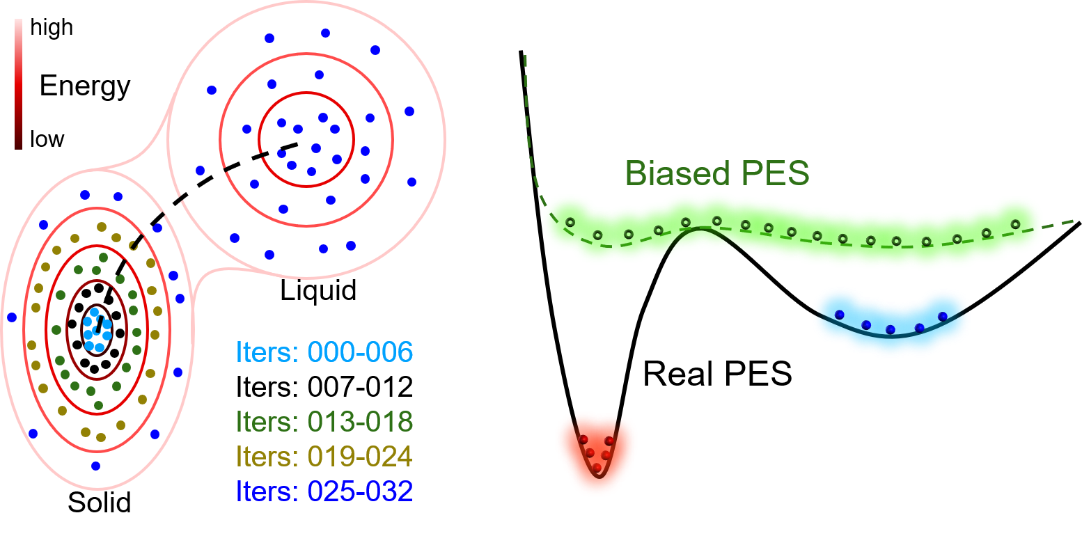
Thanks to the representation and fitting powers of machine learning models, machine learning potentials are more precise than conventional potentials. However, a coin always has two sides. There is a typical shortcoming, the low capability of extrapolation, for almost all machine learning potentials. As illustrated in the following figure, the model matches extremely well in regions covered by the dataset, while predicting wrong results in regions that have not been covered by the dataset. In this example, two atoms may be bound together un-physically due to the lack of repulsion force around the core region. Commonly, atom pairs that are extremely close to each other are not in the dataset during sampling. To avoid such unphysical binds, we can artificially design some repulsion potentials in this region, or add dimer structures into the dataset and let the model learn the repulsion by itself. 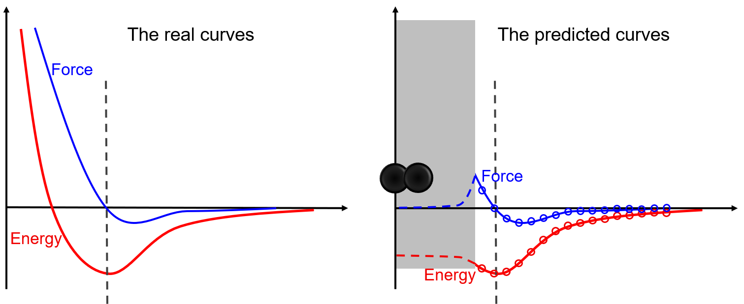Risks This is only a simple example to illustrate the risk of nonphysical phenomena that may happen in simulations if the coverage of the training dataset on the local configurational space is poor. By illustrating the risk here, we are not going to encourage people to cover the whole configurational space when training a DP model. Instead, in the section “Know the Boundaries of a Problem”, we encourage people to sample the region of the configurational space that the problem locates in. It means that training a DP model that is sufficiently accurate for the problem to be studied is OK. In principle, the configurational space may be too big to be sufficiently sampled in some cases. Then, “Training a universally robust DP model is not a trivial work if it is not impossible”.

DP-GEN

DP-GEN is the abbreviation of “Deep Potential GENerator”, which is an automatic DP model generator that is designed under the concurrent learning framework. In DP-GEN, the enrichment of the dataset and the improvement of the DP model are done concurrently. The software DP-GEN can automatically manage the whole process, including preparing job scripts (e.g. training models, exploring configurational space and examining the accuracy of the configurations, and labeling by DFT-based calculations), submitting jobs to clouds or other HPCs (high-performance clusters), and monitoring job statuses. The following figure illustrates a typical auto iteration process of DP-GEN. There are three typical processes in an iteration:

Training a group of DP models (usually four), which are then used to explore the configurational space and check whether the configurations can be well precited
Exploring configurational space by one of the DP models and examining the prediction accuracy of each configuration by comparing the prediction deviations between different DP models
Selecting some configurations with low prediction accuracy as candidates and labeling the candidate configurations by DFT-based calculations

Initially, a dataset with hundreds to thousands of DFT data is provided, and then auto iterations can be started and run continuously. The initial dataset can be generated by the DP-GEN software (e.g. by using “init_bulk”, “init_surf” modules, or even the “autotest” module), or generated by yourself. During the DP-GEN process, the coverage of the dataset on the configurational space is limited, especially in the first few iterations. As has been stated in the section of “Limitations and Risks”, the capability of a DP model trained on the dataset is also limited, which predicts a configuration accurately when the configuration is in the explored region (IR), not satisfactory when the configuration is slightly out of the boundaries of the explore region (BR), and wrong when the configuration is far away from the explored region (FR). In addition, when using a DP model to explore the configurational space (e.g. by MD), nonphysical configurations may come out when the configuration is in the FR region. To avoid selecting nonphysical configurations, only those configurations in the BR region are selected as candidates. Therefore, both lower and upper bounds of prediction errors are set to select candidate configurations. In practice, if there is a valid conventional interatomic potential, sampling can be done by using the conventional potential, which is much more robust and may get rid of nonphysical configurations. In this case, the upper bound of prediction error can be set to a relatively big one. The boundaries of the explored regions extend along with these iterations by changing sampling methods or parameters, e.g. increasing MD temperature and simulation time. DP-GEN

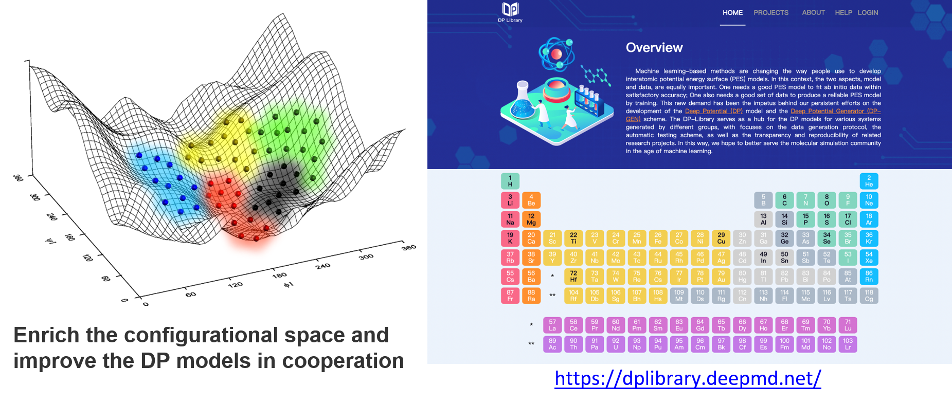
DP Library

DFT-based calculations are expansive and time-consuming. Therefore, we built the DP library to share the source DFT data to prevent waste due to recalculation, and we encourage people to contribute to it, enrich the datasets, and improve the DP models continuously. With this infrastructure, data covering different regions of the configurational space may be contributed by different researchers, as shown in the figure below. Fortunately, a DP model can be retrained and improved when the dataset is enriched. Finally, we may reach many DP models that are good enough for most of the concerned problems and can focus on applications. When we need a DP model, then we can follow the steps to check what should we do:

Check whether a trained model exists, and get the model directly from the DP library
If not, check whether any source DFT data from the DP library is valuable for you, and add some data and train a model by yourself
If neither a trained model nor any valuable data exist, start to generate the data and train the model from scratch
Contribute the source data and models to the DP library, if you are willing to

DP_LIB

Know the Physical Nature of a System

Many parameters need to be set when handling a DP project, e.g. distortion and displacement parameters for generating initial data, temperatures, pressures, simulation times, etc. when running MD simulations to explore the configurational space. Though we can copy some scripts from others and get the DP-GEN run without changing any parameters, it is not a good idea in practice. Knowing the physical nature of your system can help you to design the parameters, getting a better hands-on experience. 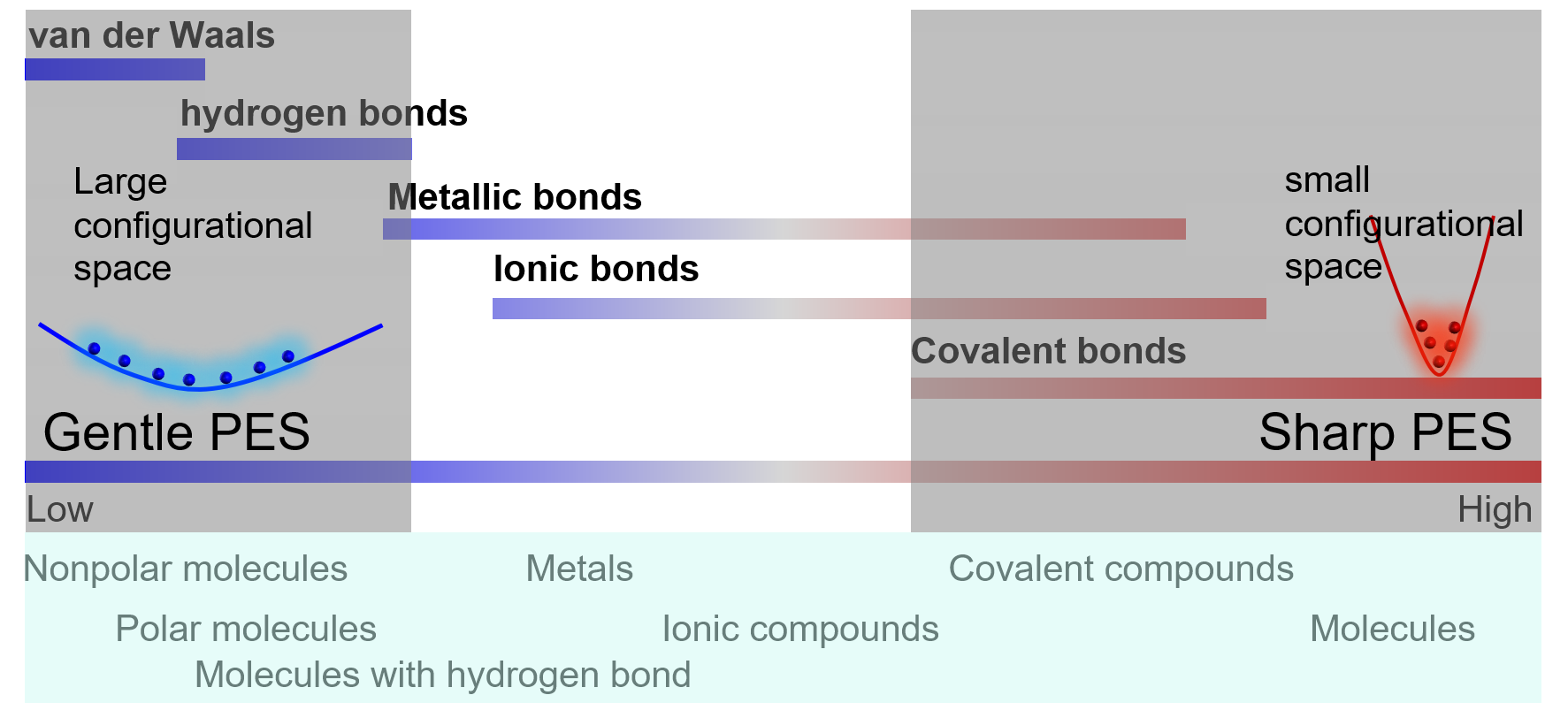The local shape of PES （potential energy surface） around a configurational space region depends on the related bond strengths. The following figure illustrates a spectrum of chemical bonds. The PES is gentle with a widespread in the configurational space for soft chemical bonds, while the PES is sharp with a localized shape for strong chemical bonds. bond_nature

Sharp regions: deep valleys in PES

the vibration of a single molecule
the vibration of atoms in a solid

Gentle regions: shallow pits in PES

movements of atoms or molecules in liquids
solid solutions

Barrier regions:

phase transformations
transition states of reactions

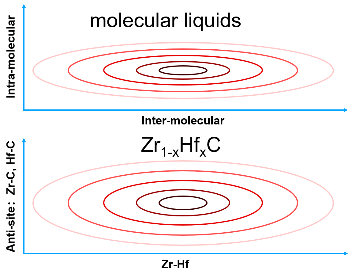
Take a molecular liquid as an example. The intra-molecular bonds will result in a sharp PES that is localized in the configurational space, where atoms vibrate around their equilibrium positions. The characteristic time of vibration is very small (~ fs). Therefore, the coverage of sampling on the configuration space may be sufficient in a short-time MD simulation. In contrast, the inter-molecular bonds will lead to a gentle PES that is spread widely in the configurational space, where molecules move around each other with a large characteristic time (~ ps). Adequate sampling in the configurational space needs long-time MD simulations, or many short-time MD simulations starting from different configurations. Similar ideas are also applicable to chemical configurational space. Take $$\rm{Zr}_{1−x}{Hf}_xC$$ as an example. It is well known that changing Zr-Hf will not change the energy significantly, which is corresponding to a gentle PES and need a lot of MC steps to sample the space. Instead, the energy of anti-site defects Zr-C or Hf-C is very high. Thus, it is possible that sampling anti-site defects is not necessary. PES For simplicity, we will take Al as an example to explain some ideas, which give the relationship between the physical properties of a material and DP-GEN parameters.

Some initial data should be generated first, for example, by using the “init_bulk” method provided in DP-GEN. In this method, we need to set the ranges of linear compression/expansion, lattice distortion, and atom displacement. Usually, for a typical solid, volume expansion from room temperature to its melting point is ~5%, which is approximately ~2% along each dimension. Therefore, setting the range of linear compression/expansion to ±2% can usually cover the boundaries of a solid well, except for the high-pressure region. Random lattice distortions can also be set to a similar value, e.g. [-3%, 3%] for each strain mode. Atom displacements may be set by referring to the bond length of the nearest neighbor (e.g. < 1%d with d being the bond length). Usually, setting to 0.01 Å is OK.
When running the auto iterations by DP-GEN, we usually sample the configurational space by MD simulations with increasing temperature and a set of pressures. The setting of temperatures can refer to the melting point of Al, Tm (~1000 K), while the setting of pressures can refer to the bulk modulus of Al, B (~80 GPa). For example, the temperatures may be set into four groups: [0.0Tm, 0.5Tm], [0.5Tm, 1.0Tm], [1.0Tm, 1.5Tm], and [1.5Tm, 2.0Tm]. In each group, a few temperatures may be selected, e.g. cutting [0.0Tm, 0.5Tm] into [0.0Tm, 0.1Tm, 0.2Tm, 0.3Tm, 0.4Tm] (In practice, 0.0Tm is useless). The pressure fluctuates during MD simulations, the magnitude of which may be ~1% of B in small systems. Then, setting the pressures being [0.00B, 0.03B, 0.06B, 0.09B] is usually sufficient. Adding -0.01B may be helpful for solids and does not set negative pressures for the liquid to avoid the risk of continuous expansion of the simulation box.
The bounds for selecting candidates (“trust_level_low” and “trust_level_high”) may depend on the strongest chemical bonds in the system, e.g. the values may be higher in molecular systems than in metals. In solids, the lower and upper bound are roughly 0.2 and 0.5 that of the RMSE (reduced mean square error) of forces, $$\sqrt{\sum f_i^2} $$. Therefore, the melting temperature or bulk modulus is also a good indication for the bounds, since the forces are proportional to these properties. For example, the “trust_level_low” of Al DP-GEN is 0.05 eV/Å, while the “trust_level_low” of W DP-GEN is 0.15 eV/Å, three times that of Al. The melting point of W (~ 3600 K) is also nearly three times that of Al (~ 1000 K). These values may be good indicators when you insert them into the spectrum shown above. However, these criteria may not suitable for molecular liquids, which need relatively higher values due to the strong intramolecular bonds, even though their melting points are low.

Know the Boundaries of a Problem

Keep in mind that “Training a universally robust DP model is not a trivial work if it is not impossible”. Usually, we only need one DP model that meets our requirements. For different tasks, the desired coverages of the dataset on configurational space are different. Following is an example to illustrate this point of view:

We are interested in the room temperature elastic properties of Al

We are further interested in the temperature dependence of elastic properties of Al

We are interested in the melting point of Al

We are further interested in the solidification process of Al

We are interested in defects (e.g. vacancies, interstitials, dislocations, surfaces, grain boundaries) of Al

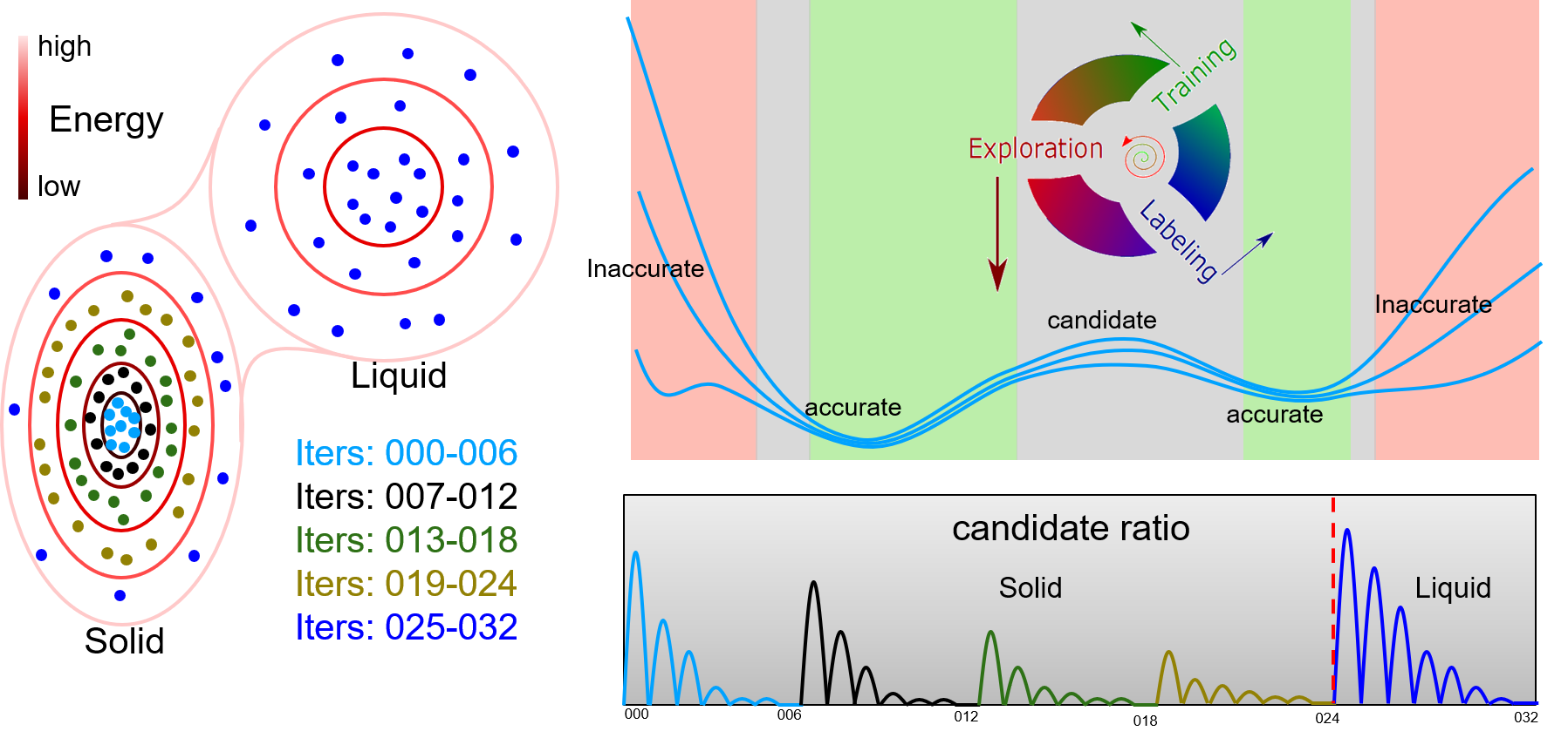
Example_Al In the first case, only configurations that are with small distortions around the equilibrium state are needed when calculating elastic properties. Therefore, only data around the equilibrium solid-state of Al are necessary. Running a DP-GEN with iterations from 000 to 006 may be enough. Additionally, if we would like to know the temperature dependence of elastic properties, iterations from 007 to 024, which further sample high energy state of Al bulk (e.g. expanded state due to thermal expansion), should be added.
In the second case, all the iterations in the figure should be done, which samples both the solid-state and liquid state of Al. However, if we are concerned about the nucleation details of Al from the liquid. The dataset may be enough (or not enough) to describe the solid-liquid interface accurately. Usually, the dataset is enough, if bonding in the material is not highly directional, e.g. for most metals. Sometimes, it is not, when bonding in the material is highly directional. For example, Ga, Si, etc. Then, an enhanced sampling method should be coupled into the DP-GEN process to sample the rare events, e.g. nucleation. For example, enforce the simulation running along the dotted line in the figure back and forth to gather samples around the saddle point.
In the third case, additional DP-GEN processes based on defect configurations (e.g. vacancies, interstitials, dislocations, surfaces, grain boundaries) are necessary. Fortunately, some local atomic configurations around defects may be similar to some distorted lattice structures or amorphous structures. Therefore, it is not necessary to explicitly include all the defect configurations during sampling. It can be seen from this simple example that a majority of efforts can be saved if the boundary of a problem can be well defined. For example, if we are only concerned about elastic properties of Al. It is not necessary to sample melts or defects, even though melts and defects are always sampled when developing DP models for metals. In contrast, when developing DP models for compounds, especially for those compounds with complex structures, melts and defects are only sampled when necessary. Therefore, before getting started with a new problem, pay some time to think about where the boundaries of the problem are and how much configurational space should be covered. When we get a new project, instead of being too excited to wait for getting into practice, plaining some milestones that are easier to achieve may facilitate the implementation of the project. For example, if our final goal is to investigate defects of Al, we can also cut the whole problem into pieces, and reach the final goal in stages, e.g. as stages 1, 2, and 3 stated above. After each stage, we can get a milestone, and then proceed to the next stage smoothly.

Gas-Phase

Simulation of the oxidation of methane

Jinzhe Zeng, Liqun Cao, and Tong Zhu

This tutorial was adapted from: Jinzhe Zeng, Liqun Cao, Tong Zhu (2022), Neural network potentials, Pavlo O. Dral (Eds.), Quantum Chemistry in the Age of Machine Learning, Elsevier. Please cite the above chapter if you follow the tutorial.

In this tutorial, we will take the simulation of methane combustion as an example and introduce the procedure of DP-based MD simulation. All files needed in this section can be downloaded from tongzhugroup/Chapter13-tutorial. Besides DeePMD-kit (with LAMMPS), ReacNetGenerator should also be installed.

Step 1: Preparing the reference dataset

In the reference dataset preparation process, one also has to consider the expect accuracy of the final model, or at what QM level one should label the data. In this paper, the Gaussian software was used to calculate the potential energy and atomic forces of the reference data at the MN15/6-31G** level. The MN15 functional was employed because it has good accuracy for both multi-reference and single-reference systems, which is essential for our system as we have to deal with a lot of radicals and their reactions. Here we assume that the dataset is prepared in advance, which can be downloaded from tongzhugroup/Chapter13-tutorial.

Step 2. Training the Deep Potential (DP)

Before the training process, we need to prepare an input file called methane_param.json which contains the control parameters. The training can be done by the following command:

$ $deepmd_root/bin/dp train methane_param.json

There are several parameters we need to define in the methane_param.json file. The type_map refers to the type of elements included in the training, and the option of rcut is the cut-off radius which controls the description of the environment around the center atom. The type of descriptor is se_a in this example, which represents the DeepPot-SE model. The descriptor will decay smoothly from rcut_smth (R_on) to the cut-off radius rcut (R_off). Here rcut_smth and rcut are set to 1.0 Å and 6.0 Å respectively. The sel defines the maximum possible number of neighbors for the corresponding element within the cut-off radius. The options neuron in descriptor and fitting_net is used to determine the shape of the embedding neural network and the fitting network, which are set to (25, 50, 100) and (240, 240, 240) respectively. The value of axis_neuron represents the size of the embedding matrix, which was set to 12.

Step 3: Freeze the model

This step is to extract the trained neural network model. To freeze the model, the following command will be executed:

$ $deepmd_root/bin/dp freeze -o graph.pb

A file called graph.pb can be found in the training folder. Then the frozen model can be compressed:

$ $deepmd_root/bin/dp compress -i graph.pb -o graph_compressed.pb -t methane_param.json

Step 4: Running MD simulation based on the DP

The frozen model can be used to run reactive MD simulations to explore the detailed reaction mechanism of methane combustion. The MD engine is provided by the LAMMPS software. Here we use the same system from our previous work, which contains 100 methane and 200 oxygen molecules. The MD will be performed under the NVT ensemble at 3000 K for 1 ns. The LAMMPS program can be invoked by the following command:

$ $deepmd_root/bin/lmp -i input.lammps

The input.lammps is the input file that controls the MD simulation in detail, technique details can be found in the manual of LAMMPS. To use the DP, the pair_style option in this input should be specified as follows:

pair_style deepmd graph_compressed.pb 
pair_coeff * * 

Step 5: Analysis of the trajectory

After the simulation is done, we can use the ReacNetGenerator software which was developed in our previous study to extract the reaction network from the trajectory. All species and reactions in the trajectory will be put on an interactive web page where we can analyze them by mouse clicks. Eventually we should be able to obtain reaction networks that consistent with the following figure.

$ reacnetgenerator -i methane.lammpstrj -a C H O --dump

The initial stage of combustion

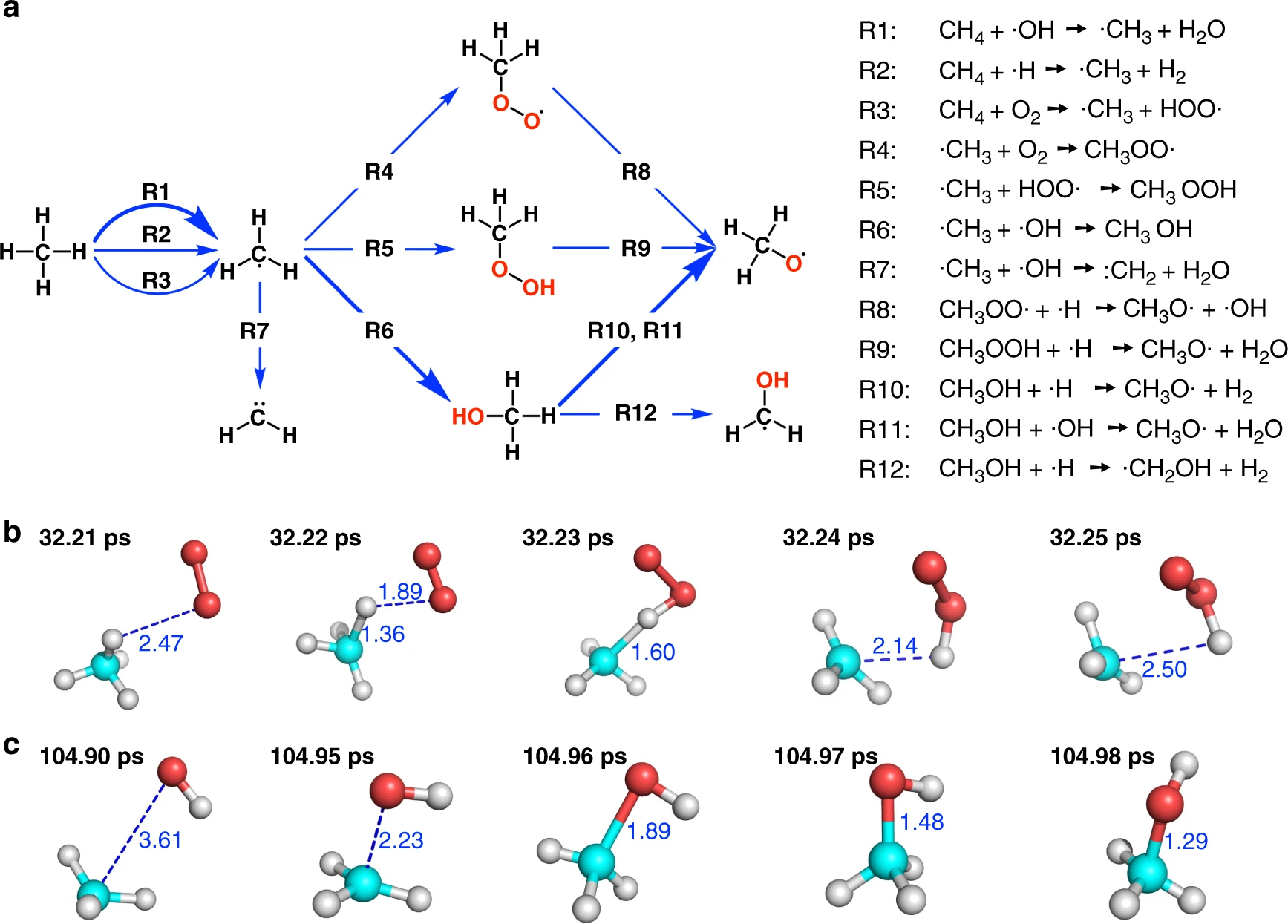
Fig: The initial stage of combustion. The figure is taken from this paper and more results can be found there.

Acknowledge

This work was supported by the National Natural Science Foundation of China (Grants No. 22173032, 21933010). J.Z. was supported in part by the National Institutes of Health (GM107485) under the direction of Darrin M. York. We also thank the ECNU Multifunctional Platform for Innovation (No. 001) and the Extreme Science and Engineering Discovery Environment (XSEDE), which is supported by National Science Foundation Grant ACI-1548562.56 (specifically, the resources EXPANSE at SDSC through allocation TG-CHE190067), for providing supercomputer time.

References

Jinzhe Zeng, Liqun Cao, Tong Zhu (2022), Neural network potentials, Pavlo O. Dral (Eds.), Quantum Chemistry in the Age of Machine Learning, Elsevier.
Jinzhe Zeng, Liqun Cao, Mingyuan Xu, Tong Zhu, John Z. H. Zhang, Complex reaction processes in combustion unraveled by neural network-based molecular dynamics simulation, Nature Communications, 2020, 11, 5713.
Frisch, M.; Trucks, G.; Schlegel, H.; Scuseria, G.; Robb, M.; Cheeseman, J.; Scalmani, G.; Barone, V.; Petersson, G.; Nakatsuji, H., Gaussian 16, revision A. 03. Gaussian Inc., Wallingford CT 2016.
Han Wang, Linfeng Zhang, Jiequn Han, Weinan E, DeePMD-kit: A deep learning package for many-body potential energy representation and molecular dynamics, Computer Physics Communications, 2018, 228, 178-184.
Aidan P. Thompson, H. Metin Aktulga, Richard Berger, Dan S. Bolintineanu, W. Michael Brown, Paul S. Crozier, Pieter J. in ‘t Veld, Axel Kohlmeyer, Stan G. Moore, Trung Dac Nguyen, Ray Shan, Mark J. Stevens, Julien Tranchida, Christian Trott, Steven J. Plimpton, LAMMPS - a flexible simulation tool for particle-based materials modeling at the atomic, meso, and continuum scales, Computer Physics Communications, 2022, 271, 108171.
Denghui Lu, Wanrun Jiang, Yixiao Chen, Linfeng Zhang, Weile Jia, Han Wang, Mohan Chen, DP Train, then DP Compress: Model Compression in Deep Potential Molecular Dynamics, 2021.
Jinzhe Zeng, Liqun Cao, Chih-Hao Chin, Haisheng Ren, John Z. H. Zhang, Tong Zhu, ReacNetGenerator: an automatic reaction network generator for reactive molecular dynamics simulations, Phys. Chem. Chem. Phys., 2020, 22 (2), 683–691.

Learning Resources

Here is the learning Resources:

Video Tutorials（Chinese)

Some Video Resources：

Basic theoretical courses:

DeePMD-kit and DP-GEN

Writing Tips

Hello volunteers, this docs tells you how to write articles for DeepModeling tutorials.

You can just follow 2 steps:

Write in markdown format and put it into proper directories.
Change index.rst to show your doc.

Write in Markdown and Put into proper directories.

You should learn how to write a markdown document. It is quite easy!

Here we recommend you 2 website:

You should know the proper directories.

Our Github Address is: https://github.com/deepmodeling/tutorials

All doc is in: “source” directories. According to your doc’s purpose, your doc can be put into 4 directories in “source”:

Tutorials: Telling beginners how to run Deepmodeling projects.
Casestudies: Some case telling people how to use Deepmodeling projects.
Resources: Other resources for learning.
QA: Some questions and answers.

After that, you should find the proper directories and put your docs.

For example, if you write a “methane.md” for case study, you can put it into “/source/CaseStudies/Gas-phase”.

Change indexs.rst to show your doc.

Then you should change the index.rst to show your doc.

You can learn rst format here: reStructuredText

In short, you can simply change index.rst in your parent directories.

For example, if you put “methane.md” into “/source/CaseStudies/Gas-phase”, you can find and change “index.rst” in “source/CaseStudies/Gas-phase”. All you should do is imitating such file. I believe you can do it!

If you want to learn more detailed information about how to build this website, you can check this:

Q & A

here is Q & A

Discussions and Feedbacks:

The tutorials need feedbacks from you. If you think some tutorials are confused, please write your feedbacks on our discussion board.

Working Now:

At present, we are writing tutorials for:

DeePMD-kit
DP-GEN

Another team focus on writing some brief materials about AI + Science for beginners, such as:

What is machine learning
What is MD(Molecular Dynamics)
The core concept about AI + Science

Welcome to DeepModeling Tutorial!

Using DeePMD-Kit

Introduction

Installation

Install off-line packages

Install with conda

Install with docker

Theory

How to Setup a DeePMD-kit Training within 5 Minutes

Tutorial Data

Preparing Data

Training

Freeze/Compress the Model

Handson-Tutorial(v2.0.3)

Data preparation

Training

Prepare input script

Train a model

Freeze and Compress a model

Test a model

Run MD with LAMMPS

Using DP-GEN

Hands-on tutorial for DP-GEN (v0.10.3)

General Introduction

Input files

Run process

param.json

Basics keywords (Line 2-3):

Data-related keywords (Line 4-10):

Training-related keywords (Line 12-58):

Exploration-related keywords (Line 59-69):

Labeling-related parameters (Line 70-76):

Output files

00.train

01.model_devi

02.fp

Practical-Guidelines-for-DP

Practical Guidelines for DP

Know the Toolbox Well

Deep Potential

Configurational Space

Sampling Methods

Limitations and Risks

DP-GEN

DP Library

Know the Physical Nature of a System

Know the Boundaries of a Problem

Gas-Phase

Simulation of the oxidation of methane

Step 1: Preparing the reference dataset

Step 2. Training the Deep Potential (DP)

Step 3: Freeze the model

Step 4: Running MD simulation based on the DP

Step 5: Analysis of the trajectory

Acknowledge

References

Learning Resources

Some Video Resources：

Basic theoretical courses:

DeePMD-kit and DP-GEN

Writing Tips

Write in Markdown and Put into proper directories.

Change indexs.rst to show your doc.

Q & A

Discussions and Feedbacks:

Working Now:

Indices and tables